How to read graphs: functions, surfaces and probability

A graph can be drawn correctly and still be read incorrectly. An intersection is not necessarily a root, a surface can hide a valley behind a peak, and the height of a bell curve is not a probability. Getting an image onto the screen is only the beginning: the useful part is understanding what it tells you.

Start with three questions. What do the axes represent? Which quantities can change? What relationship are you trying to test? We will apply those questions to a function, a surface and a normal distribution, using examples you can explore in Algor Graphs.

Read the axes before the curve

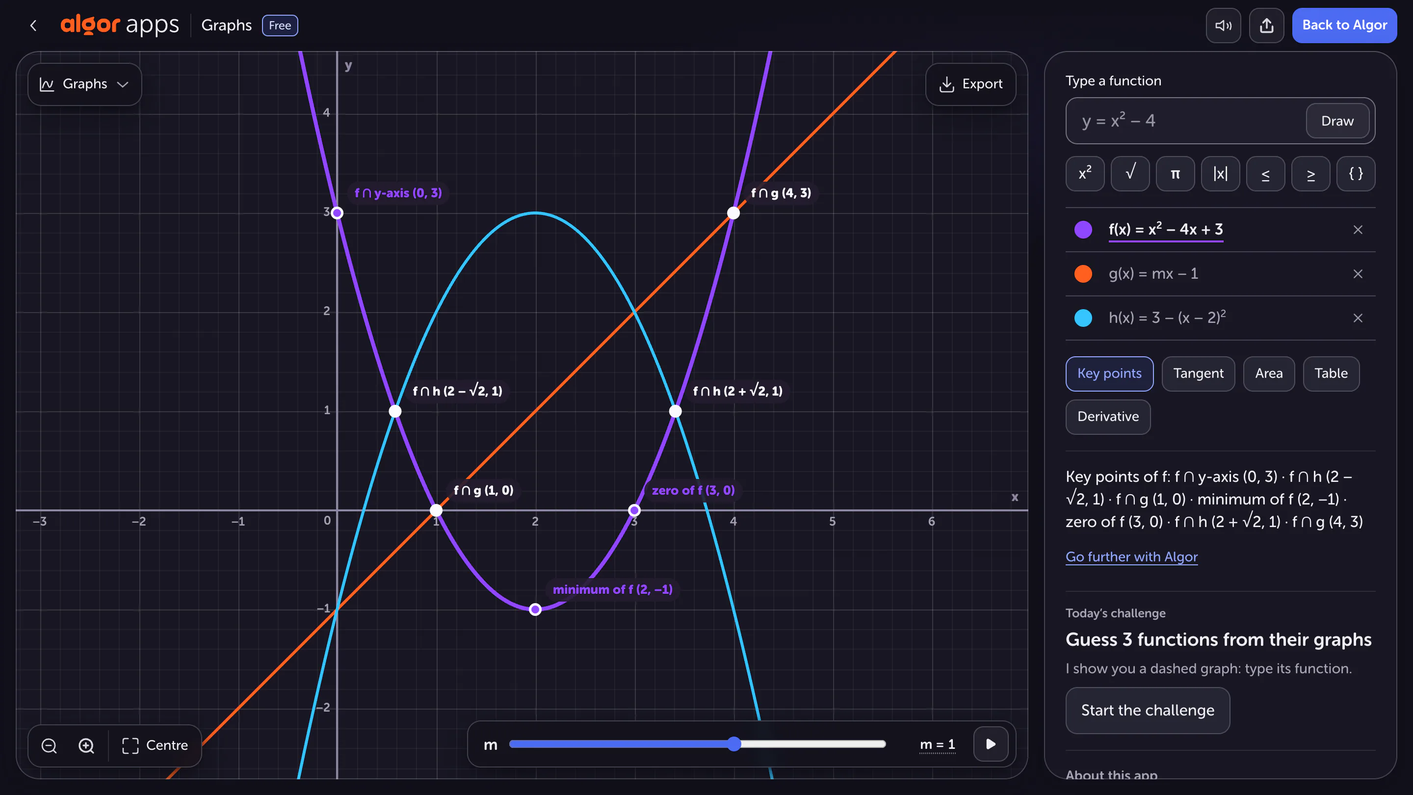
On a Cartesian plane, a point (x, y) pairs an input with its corresponding function value. For y = x² − 4x + 3, the point (0, 3) tells you that f(0) = 3. It does not mean that 3 is a root. Roots occur where the output is zero, so they belong on the horizontal axis.

Check the scale as well. A parabola can look narrower after a change in the display's proportions even though its equation is unchanged. Before comparing screenshots, inspect the values on both axes. For an applied problem, include units: seconds and metres give a graph a different meaning from two unspecified variables. A correct numerical answer can still be a poor interpretation if you have lost track of the quantities being compared.

Separate roots, vertices and intersections

Factor f(x) = x² − 4x + 3 as (x − 1)(x − 3), and its roots are immediately visible: 1 and 3. Complete the square to obtain (x − 2)² − 1, and you can identify the vertex (2, −1). These calculations answer different questions: where the function is zero and where it reaches its minimum.

Now add g(x) = x − 1. Intersections satisfy f(x) = g(x), giving x² − 5x + 4 = 0. The solutions are x = 1 and x = 4; substitution into the line gives (1, 0) and (4, 3). Only the first intersection is also a root of f. The second is a useful reminder that an intersection between two graphs need not lie on either axis.

Predict a change before moving a slider

The line y = mx − 1 isolates the effect of slope. Changing m changes the line's inclination, while its vertical intercept stays at (0, −1). Before moving from m = 1 to m = 2, predict what will happen at x = 1. Then compare the graph with your calculation.

This turns an animation into an exercise. Moving sliders without a question can produce attractive pictures without clarifying how coefficients affect behaviour. Change one parameter at a time, and write a sentence about what stayed fixed. If your prediction was wrong, record both the mistaken step and the check that corrected it in an exam error log.

A surface gives height from two inputs

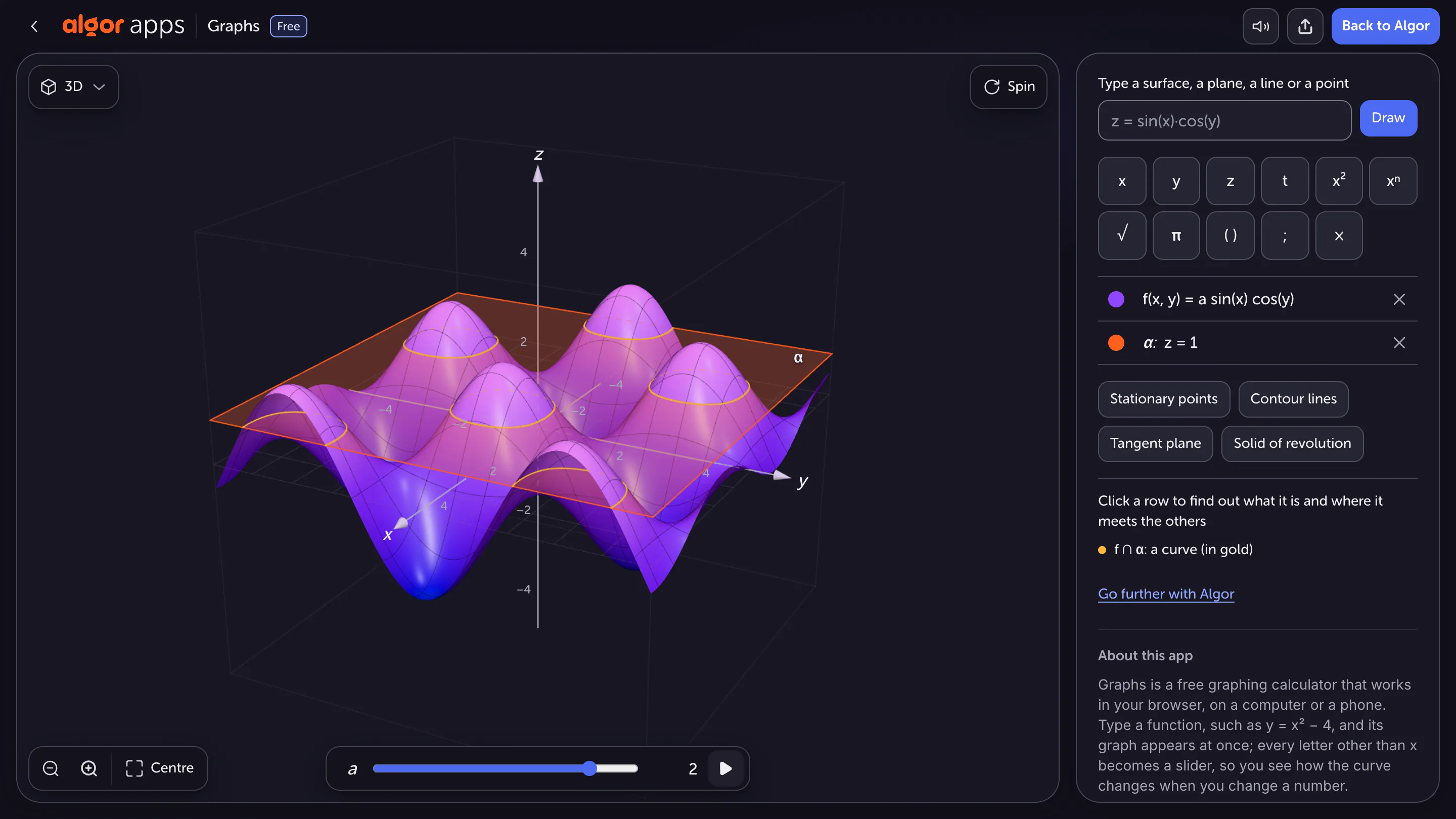
For z = f(x, y), you choose two input coordinates and obtain a height. The surface z = a·sin(x)·cos(y) describes how z varies across a plane; it is not simply an ordinary curve viewed from another angle. In the screenshot, a = 2 and the orange plane is z = 1.

Their intersection consists of points satisfying 2·sin(x)·cos(y) = 1. You are seeing a level curve at its actual height. Consider a limiting case: when a = 0, the entire surface lies in z = 0, so it no longer meets the plane z = 1. That prediction tells you something precise about the parameter, beyond what a particular viewing angle happens to reveal.

Under a normal curve, read the area

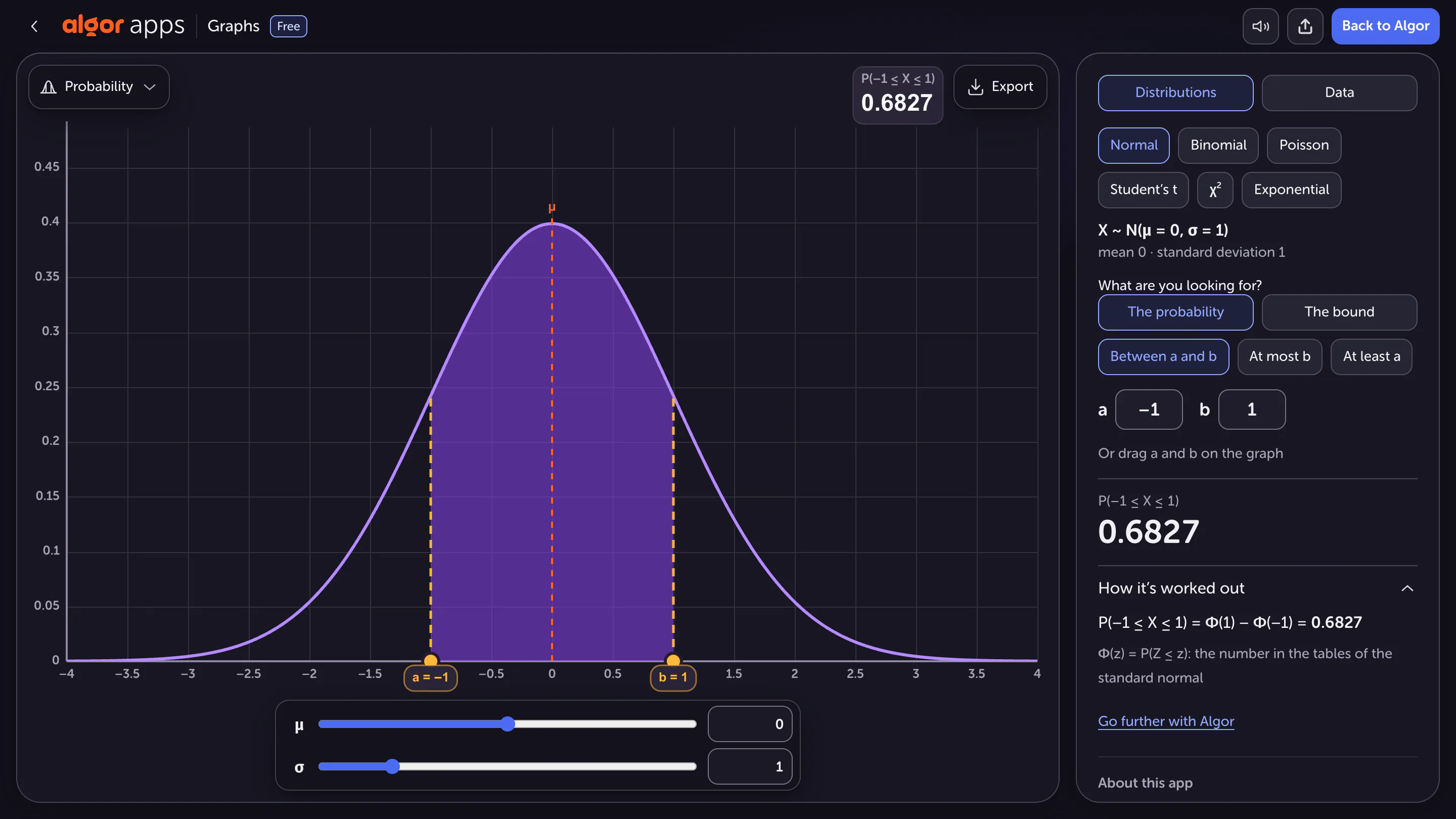
A standard normal variable has mean 0 and standard deviation 1. The probability of a value between −1 and 1 is the area beneath the curve over that interval: approximately 0.6827, or 68.27%. This number describes a proportion of the total area, not the height of the central point.

The curve is a probability density. For a continuous variable, an individual exact value has probability zero, whereas an interval can have positive probability. Widen the interval symmetrically and its area increases; bring the endpoints together and its area decreases. The total area beneath the complete curve is 1. Locating the peak alone does not answer an interval question.

Worked example: move from the middle to the tails

Suppose a question asks for the probability that a standard normal variable falls outside the interval from −1 to 1. In Algor Graphs, start with the central region already displayed and translate the request: you want values below −1 or above 1. These are two separate regions, not a rectangle drawn over the curve.

The total area is 1 and the central area is approximately 0.6827. The required probability is therefore 1 − 0.6827 = 0.3173, or about 31.73%. This calculation uses the complement of the central event: everything left outside the selected interval. Write the event beside your answer so you do not confuse this number with the probability of being in the middle.

The two tails have equal areas because the distribution is symmetric about zero. Each tail therefore has an area of approximately 0.15865. If the question asked only about values greater than 1, the answer would be about 15.87%, not 31.73%.

Check your interpretation in three steps

Try explaining each image without referring to its colours. For the plane graph, state the equation that defines an intersection. For the surface, identify the two inputs and explain what the cutting plane represents. For the normal distribution, turn the shaded region into a sentence that includes both an interval and a probability.

Sources and further reading

• OpenStax · Quadratic functions
• OpenStax · Introductory Statistics 2e