How to learn physics with simulations: predict, calculate, explain

A physics simulation can make a field visible, trace a light ray or display a force. The challenge is turning what happens on screen into an explanation. Start with a specific question: what will change if you alter one quantity, and which physical law lets you predict the result?

Use three examples from Algor's Physics simulations: an electric field, a converging lens and an inclined plane with friction. Write your prediction before moving the controls, compare it with the outcome and explain any difference. This makes the simulation a test of your reasoning rather than a sequence of attractive movements.

An electric field is a vector

An electric field describes force per unit positive test charge: E = F/q. It has direction as well as magnitude. Arrows in a field diagram represent these properties. They are not particles emerging from a charge, nor are they compulsory trajectories followed by every object placed in the field.

For two equal positive charges, the field at their midpoint cancels by symmetry. The two contributions have equal magnitudes and opposite directions. That does not mean the source charges produce no fields. Their vector sum is zero at that particular point. Moving elsewhere does not guarantee the same cancellation. Always distinguish a contribution from the resultant of several contributions.

Change distance while keeping other conditions fixed

For an isolated point charge, field magnitude varies as 1/r². Doubling the distance r, with everything else unchanged, reduces the field to one quarter. With several charges, you must add their vector contributions. Applying the inverse-square rule to one distance alone does not describe the complete system.

Also distinguish field from force. The field depends on the source charges; the force on a test charge is F = qE. A negative test charge experiences a force opposite to the field's direction. Write down that distinction before interpreting arrows that might refer to different quantities. A diagram becomes much easier to read when every arrow has a named physical meaning.

A lens involves three clearly defined distances

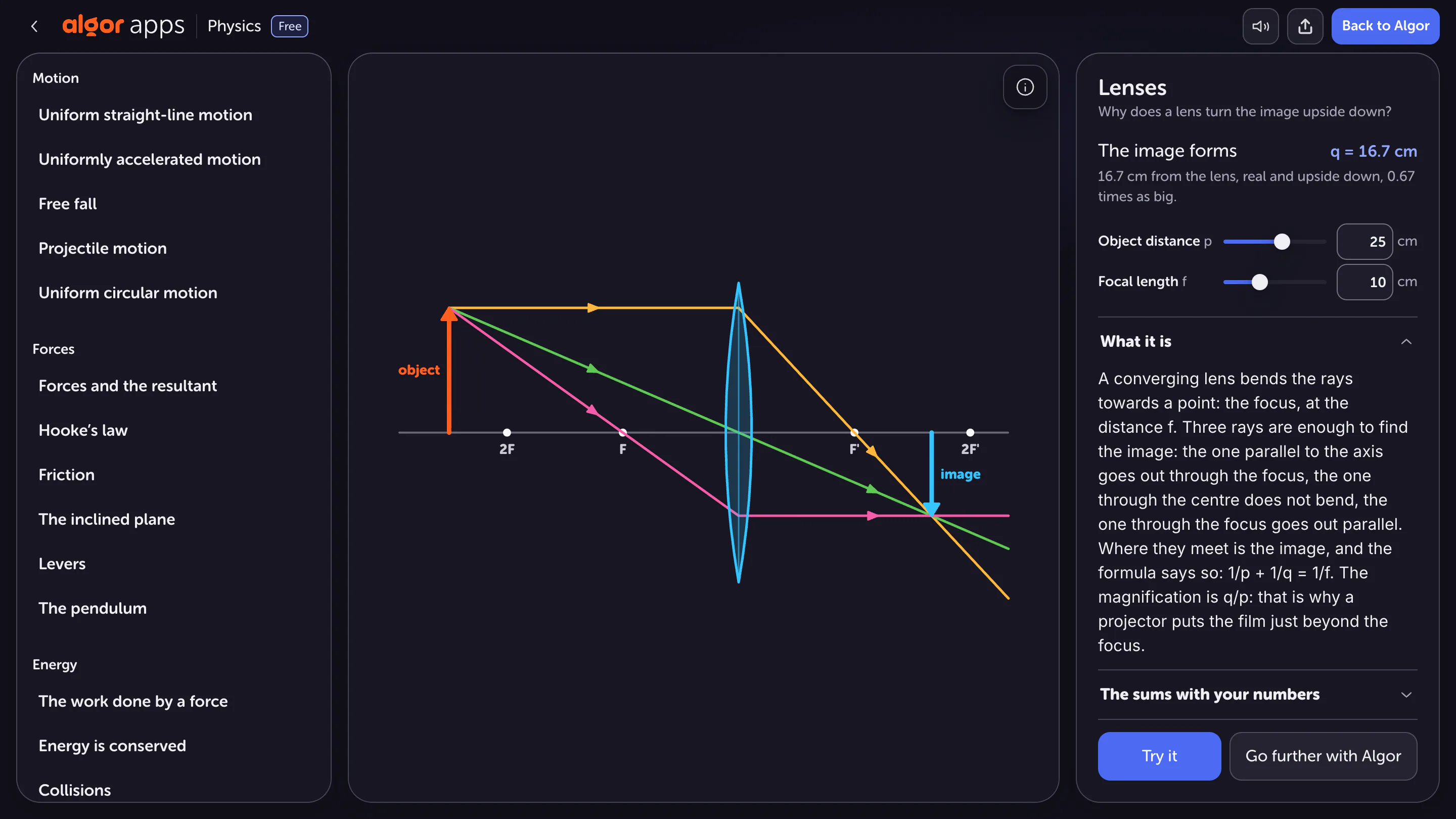
For a thin converging lens in the paraxial model, 1/f = 1/dₒ + 1/dᵢ. With focal length f = 10 cm and object distance dₒ = 25 cm, you obtain 1/dᵢ = 1/10 − 1/25 = 3/50. The image therefore forms approximately 16.7 cm from the lens on its other side.

Magnification is m = −dᵢ/dₒ, approximately −0.67. The negative sign indicates an inverted image. A magnitude below 1 indicates an image smaller than the object. These are two separate pieces of information contained in the same result. The minus sign does not mean that an object has a physically negative size.

Follow the rays and remember the assumptions

Principal rays help construct the image position. A ray parallel to the axis passes through the focus after an ideal converging lens. A ray through the optical centre is approximated as undeviated. Their intersection helps identify the image's position and orientation.

This construction assumes an ideal lens and rays close to the axis. It does not automatically account for aberrations, real lens thickness or every effect in a camera system. When moving the object closer, make a new prediction and distinguish positions beyond the focal point, at the focal point and inside the focal distance. The familiar diagram is one case within a larger set of possibilities.

Resolve weight on an inclined plane

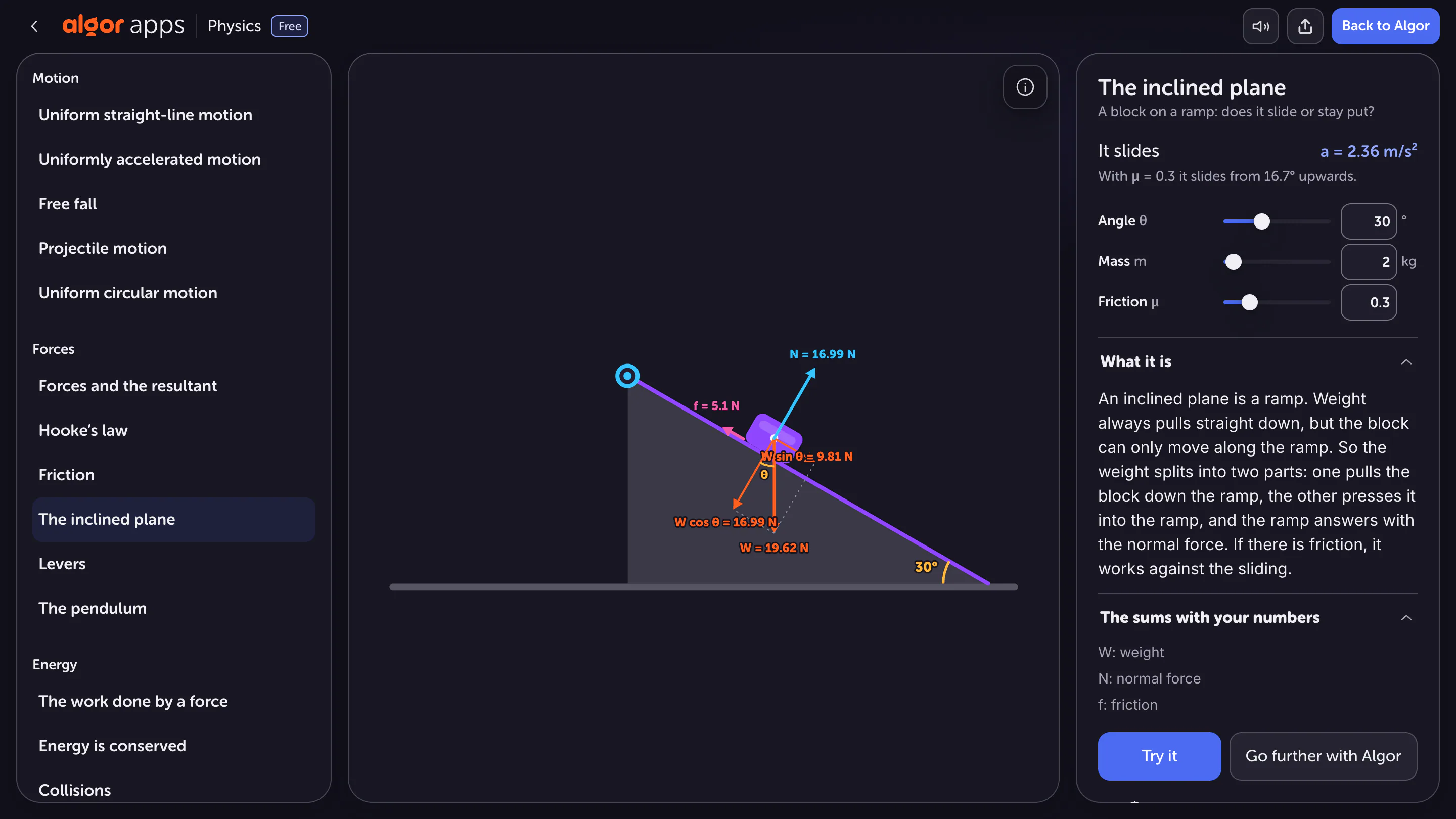
For mass m on a plane inclined at angle θ, weight mg has components mg·sinθ along the plane and mg·cosθ perpendicular to it. In the simple case without other perpendicular forces, the normal reaction is N = mg·cosθ. It is not equal to the entire weight except when the plane is horizontal.

For m = 2 kg, θ = 30° and g = 9.81 m/s², the downslope component is about 9.81 N and the normal reaction about 16.99 N. If the object is sliding and its coefficient of kinetic friction is 0.3, friction is about 5.10 N. Its resulting acceleration down the plane is approximately 2.36 m/s². With friction removed and the slope unchanged, acceleration would become g·sin(30°), about 4.91 m/s². This comparison isolates the effect of the friction term.

Static and kinetic friction are different

Before sliding starts, static friction adjusts up to a maximum μₛN. It does not always equal μₛN. During sliding, the elementary model instead uses kinetic friction μₖN, opposing relative motion. Applying the previous numerical calculation therefore requires you to identify which situation is being studied.

If a simulation provides a generic friction coefficient, state the interpretation you use in your solution. A correct formula applied to the wrong motion state can produce an incorrect explanation. Identify the motion and the forces first, then substitute the numbers. This order also makes it easier to recognise when an assumption has changed between two trials.

Keep the prediction and the correction

In an exam error log, record a prediction, the equation used, the result and one modelling assumption for each scene. Check vector addition for the field, the meaning of the sign for the lens and the friction regime for the inclined plane.

Close the tool and alter one value on paper. If you can predict the direction of the change before calculating its numerical size, you have a physical explanation that the simulation can test. Reopen it to investigate that prediction, then describe why the result agrees or where your reasoning needs revision.

Sources and further reading

• OpenStax · Inclined planes
• OpenStax · Thin lenses
• OpenStax · Friction